
The Climate Change Hazards Information Portal (CCHIP) provides visualized historical and projected climate data and analyses for sectors including but not limited to Infrastructure, Emergency Management, Agriculture, Natural Resources, Public Health, and Insurance interests. It is designed to provide ready access to customized climate information based on quality controlled data drawn from various sources and packaged in a ‘one-stop’ location. Its highly practical features include direct linkages to location-specific, infrastructure climate design values (from Canadian codes and standards) as well as information on key agricultural thresholds and the ability to quickly customize analyses relative to particular threshold settings and time periods.
While CCHIP is designed for ease of use and can be manipulated by users with little or no climate knowledge, for important decision-making purposes CCHIP should always be used in conjunction with the appropriate scientific and technical expertise.
In this respect, Risk Sciences International (RSI) provides customized analytical support for our clients, at minimal cost, by highly experienced staff (see supporting staff below). Professional climatological, meteorological, engineering and other domain-specific services can help ensure CCHIP outputs are correctly interpreted and applied.
RSI assumes no responsibility for users’ mis-interpretation or mis-application of data and analyses obtained through CCHIP.
CCHIP eliminates the need for the user to search for, collect, apply quality control and independently compute statistics based on climate data for their location(s) of interest. For locations with minimal data, other options (e.g., gridded datasets) are available for use.
The location bar will recognize virtually any location in Canada, whether by place name, postal code, or by the name of a formal meteorological observation station. Specifying an approximate location is usually sufficient, since CCHIP will automatically suggest the nearest meteorological stations as optional data sources for the user. Start typing in the location and the system will begin filling in locations in our database. Click on the proper location from the list to select it. Let us know if your town or area is not in the system!
This option may not be available to you, or may be auto-selected according to your licence, directing/limiting you to those variables of most common interest within the sector or sectors covered by your licensing agreement. CCHIP filters variables by sector to deliver what is typically most meaningful for users in the identified sector(s).
If your CCHIP license is not sector specific, then you would select your area of focus here.
CCHIP automatically selects the nearest meteorological station when users enter a (new) location. However, it is important to recognize that the nearest station will not always be the best station to use. This may be the case if a station has incomplete records, or if its location is non-climatologically representative of the users' specified location (despite being closest to it). Most basic parameters of daily temperature and precipitation are generally available. Data for certain climate elements (such as wind for example) and for certain variables (such as short duration rainfall intensities) are typically available for airport locations only.
Generally speaking, CCHIP covers all of Canada.
If a no data message appears for a particular meteorological station and climate variable, users are encouraged to search for an alternative station with more complete data. This can be done by clicking on the nearby station list at the top right of the dashboard.
Stations listed as Data Sources are categorized by colour: stations containing more than 30 years of records are colour-coded in green, those with 15 to 30 years of data are yellow, and those with fewer than 15 years of data are coloured red.
Depending on the users’ period of study, the stations with data for the relevant years should be picked. It is highly recommended to use stations with the longest period of record for climate analyses, since these stations will most properly reflect the ‘long term’ climate of a location. Please note that stations with near-complete data for the years 1981 to 2010 are suitable for climate change projection analyses. To establish a ‘climatology’ of the region, a longer-term dataset is preferred, however even shorter duration stations can provide some information about the incidence of climate extremes.
RSI can provide assistance for locations with limited data. Contact us for assistance.
CCHIP obtains its historical data from Environment and Climate Change Canada (ECCC) and Natural Resources Canada (gridded data). Daily data are available for analysis, but full availability varies among stations depending upon what was originally collected. We are working to incorporate hourly data collected from major meteorological stations across Canada (primarily airport locations) and many of these stations are completed. CCHIP currently contains daily data up to the end of 2016, although updates are continuously underway. As part of the licence for the tool, regular updates of data are ensured.
CCHIP relies on ECCC Climate Data Archive for its historical data (hundreds of stations over various periods of record). The data provided by ECCC is provided ‘as-is’ and is vetted by that organization. Errors or omissions in the ECCC dataset may therefore also be present in the CCHIP dataset, although effort has been made to recheck values in our database.
Although CCHIP primarily relies on data from ECCC, customized climate datasets can be incorporated into the system from clients and provide calculations and graphing just like ECCC stations. Ask about this feature if of interest, and note this additional station data would only be available to the user supplying it — not the entire CCHIP subscriber base.
Also sourced from ECCC are high-frequency precipitation measurements which are collected by tipping bucket rain gauges. These data are known as ‘Intensity-Duration-Frequency’ (IDF) data. CCHIP selects and shows stations with IDF data as well and they are labelled with the ‘+IDF’ in their name. Information on IDF data from ECCC can be found here.
Additionally, high-resolution (10km by 10km) peer-reviewed and vetted gridded observed data that cover the entire Canadian landmass (particularly useful in areas with poor ECCC station coverage) is provided within CCHIP. The gridded dataset is known as CANGRD and was developed in a collaboration between Natural Resources Canada and ECCC, led by D. McKenney (2011). You may select CANGRD as a data source just as you would select an observation station. Although this dataset is well accepted and researched, a real observation station, where available, may be preferable. In very remote locations however, CANGRD may be the only acceptable data source. A website with details on the development of the gridded dataset can be found here.
Official Intergovernmental Panel on Climate Change (IPCC) assessments predominantly rely on international research centres to contribute Global Climate Model (GCM) projection information. CCHIP uses GCM projection data from the same set of models. The most recent assemblage of GCM projections was provided for the IPCC 5th assessment of 2013 (AR5). In this assessment, 40 GCMs were used with multiple runs per model, resulting in approximately 75 projection estimates from which to calculate possible future conditions. Maximum, minimum and mean temperature are standard output variables from these GCMs, as is precipitation.
The suite of models used in AR5 is from the Fifth Coupled Model Intercomparison Project (CMIP5), coordinated by the World Climate Research Program. The AR5 data used by CCHIP were retrieved from this site.
The GCMs and individual runs which produced the data used by CCHIP are indicated in the table below.
| Mod (# of runs) | Organization | Country | Organization Details |
|---|---|---|---|
| ACCESS1-0 (1) | CSIRO-BOM | Australia | CSIRO (Commonwealth Scientific and Industrial Research Organisation, Australia), and BOM (Bureau of Meteorology, Australia) |
| ACCESS1-3 (1) | CSIRO-BOM | Australia | CSIRO (Commonwealth Scientific and Industrial Research Organisation, Australia), and BOM (Bureau of Meteorology, Australia) |
| BCC-CSM1-1 (1) | BCC | China | Beijing Climate Center, China Meteorological Administration |
| BCC-CSM1-1-M (1) | BCC | China | Beijing Climate Center, China Meteorological Administration |
| BNU-ESM (1) | GCESS | China | College of Global Change and Earth System Science, Beijing Normal University |
| CanESM2 (5) | CCCma | Canada | Canadian Centre for Climate Modelling and Analysis |
| CCSM4 (6) | NCAR | US | National Center for Atmospheric Research |
| CESM1-BGC (1) | NSF-DOE-NCAR | US | National Science Foundation, Department of Energy, National Center for Atmospheric Research |
| CESM1-CAM5 (3) | NSF-DOE-NCAR | US | National Science Foundation, Department of Energy, National Center for Atmospheric Research |
| CMCC-CESM (1) | CMCC | Italy | Centro Euro-Mediterraneo per I Cambiamenti Climatici |
| CMCC-CM (1) | CMCC | Italy | Centro Euro-Mediterraneo per I Cambiamenti Climatici |
| CMCC-CMS (1) | CMCC | Italy | Centro Euro-Mediterraneo per I Cambiamenti Climatici |
| CNRM-CM5 (1) | CNRM-CERFACS | France | Centre National de Recherches Meteorologiques / Centre Europeen de Recherche et Formation Avancees en Calcul Scientifique |
| CSIRO-Mk3-6-0 (10) | CSIRO-QCCCE | Australia | Commonwealth Scientific and Industrial Research Organisation in collaboration with the Queensland Climate Change Centre of Excellence |
| FGOALS-g2 (1) | LASG-IAP | China | LASG, Institute of Atmospheric Physics, Chinese Academy of Sciences |
| FGOALS-s2 (1) | LASG-IAP | China | LASG, Institute of Atmospheric Physics, Chinese Academy of Sciences |
| FIO-ESM (3) | FIO | China | The First Institute of Oceanography, SOA, China |
| GFDL-CM3 (1) | NOAA GFDL | US | Geophysical Fluid Dynamics Laboratory |
| GFDL-ESM2G (1) | NOAA GFDL | US | Geophysical Fluid Dynamics Laboratory |
| GFDL-ESM2M (1) | NOAA GFDL | US | Geophysical Fluid Dynamics Laboratory |
| GISS-E2-H (1) | NASA GISS | US | NASA Goddard Institute for Space Studies |
| GISS-E2-H-CC (1) | NASA GISS | US | NASA Goddard Institute for Space Studies |
| GISS-E2-R (1) | NASA GISS | US | NASA Goddard Institute for Space Studies |
| HadGEM2-AO (1) | MOHC | UK | MetOffice Hadley Centre (additional HadGEM2-ES realizations contributed by Instituto Nacional de Pesquisas Espaciais) |
| HadGEM2-CC (3) | MOHC | UK | MetOffice Hadley Centre (additional HadGEM2-ES realizations contributed by Instituto Nacional de Pesquisas Espaciais) |
| HadGEM2-ES (4) | MOHC | UK | MetOffice Hadley Centre (additional HadGEM2-ES realizations contributed by Instituto Nacional de Pesquisas Espaciais) |
| INMCM4 (1) | INM | Russia | Institute for Numerical Mathematics |
| IPSL-CM5A-LR (4) | IPSL | France | Institut Pierre-Simon Laplace |
| IPSL-CM5A-MR (1) | IPSL | France | Institut Pierre-Simon Laplace |
| IPSL-CM5B-LR (1) | IPSL | France | Institut Pierre-Simon Laplace |
| MIROC-ESM (1) | MIROC | Japan | Japan Agency for Marine-Earth Science and Technology, Atmosphere and Ocean Research Institute (The University of Tokyo), and National Institute for Environmental Studies |
| MIROC-ESM-CHEM (1) | MIROC | Japan | Japan Agency for Marine-Earth Science and Technology, Atmosphere and Ocean Research Institute (The University of Tokyo), and National Institute for Environmental Studies |
| MIROC5 (3) | MIROC | Japan | Atmosphere and Ocean Research Institute (The University of Tokyo), National Institute for Environmental Studies, and Japan Agency for Marine-Earth Science and Technology |
| MPI-ESM-LR (3) | MPI-M | Germany | Max Planck Institute for Meteorology (MPI-M) |
| MPI-ESM-MR (1) | MPI-M | Germany | Max Planck Institute for Meteorology (MPI-M) |
| MRI-CGCM3 (1) | MRI | Japan | Meteorological Research Institute |
| NorESM1-M (1) | NCC | Norway | Norwegian Climate Centre |
With increased computing power, a greater number of atmospheric phenomena have been incorporated into GCMs, and the models’ spatial and temporal resolutions have improved (Kharin et al., 2013). There has also been a large increase in the availability of model outputs and the ability to produce projections of future climate based upon an ‘ensemble’ of many models. These two factors give us a generally greater level of confidence in the projected values of climate parameters. CCHIP uses all available AR5 model runs (many models have more than a single projection available), and these are used together with baseline climate observations to generate measures of future conditions (described in the ‘methodology’ section of this document). The use of multiple models to generate a ‘best estimate’ of climate change is preferred over a single model outcome. Research has indicated that the use of multi-model ensembles is preferable to the selection of a single or few individual models since each model can contain inherent biases and weaknesses (IPCC-TGICA, 2007; Tebaldi and Knutti, 2007).
The use of many model estimates allows for the calculation of central tendencies as well as the range of future values. Based on the ‘spread’ of these models, different characterisations of uncertainty can be provided. Simply put: a variable which shows less spread among many models is more reliable than a variable which has a very large range of projected outcomes. This is critical in the consideration of uncertainty. Beneath charts with model projections, CCHIP provides ‘box and whisker’ plots and tables (downloadable) of the full range of all model run projections. The top horizontal bar is the highest model value, the bottom horizontal bar is the lowest model value, the box represents the range of 50% of the models with the top being the 75th percentile value, the bottom being the 25th percentile value. The median is represented by the horizontal line in the centre of the shaded box. The projected value from each GCM can be seen by the CCHIP user hovering the mouse over each data point, or by consulting the summary tables which are downloadable beneath the boxplot.
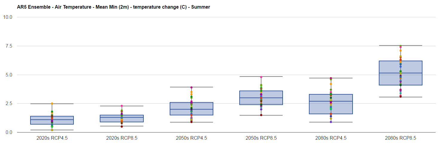
An example of box-and-whisker plot in CCHIP, showing the spread of the GCM data values
A new initiative in the IPCC AR5 was the introduction of RCPs (Representative Concentration Pathways). They represent a range of possible projection outcomes which depend upon different emission rate assumptions which generate different degrees of atmospheric warming. The lowest RCP 2.6, represents an increase of 2.6 W/m2 to the system, while the highest RCP 8.5 represents an increase of 8.5 W/m2 of energy. This range encompasses the best estimate of what is possible under a small perturbation situation (2.6) and under a large increase in warming (8.5). Within CCHIP, both the 4.5 (moderate) and 8.5 (high) projected change are presented as future emission pathways and the resulting projections are based on these two alternatives. It is unknown which of the RCPs will apply in the future. However, it is important to note that historically, the GHG emissions have followed the highest (8.5) pathway. In the absence of a meaningful global agreement on GHG reduction, this trend is expected to continue which would support this pathway going forward.
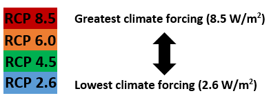
RCP levels illustration
The delta approach is one of several methods which can be used to obtain downscaled projections of future climate. It is perhaps the simplest approach, the easiest to understand, and has been widely used for impacts and adaptation studies. Is has also been shown to compare well with the accuracy of other approaches. When this method is coupled with the use of many models to generate projections, it generally provides more useful information than when a single or small set of models are used, regardless of their spatial or temporal resolution.
In the past, model data were difficult to obtain and process, making it challenging to use the delta approach together with a large ensemble of models. Modern data storage capacity and computing power allow CCHIP to apply the delta approach using outputs from all 40 GCMs and all model runs used in the IPCC AR-5.
The following 5 steps summarize CCHIP’s process for providing future estimates of climate variables:
CCHIP provides projections of variables for which data are available with acceptable levels of confidence. This is why some variables presented within CCHIP may not have projected values. Please contact us for questions about specific non-projected variables if interested.
CCHIP allows for the inclusion in users' analyses of key climate design and agroclimatic thresholds, by making available select information from national infrastructure codes and standards and the agricultural literature, respectively. Based on the users' indicated location and sector of interest, CCHIP provides reference to all potentially relevant codes, standards, and crop climate requirements, allowing the user to retrieve and plot threshold values specific to their location and the asset or crop type of concern. Look for the ‘info’ icon next to the sector selection.
Infrastructure climate design values are currently provided from the National Model Building Code of Canada and all relevant codes and standards of the Canadian Standards Association (CSA), Additional climate design information, for further national codes and standards of Canada, are planned for future versions of CCHIP.
Sources of crop growth thresholds are cited together with each crop-specific value provided within CCHIP.
Your invitation to use CCHIP includes a CCHIP 101 Webinar, to be scheduled by your committee chair (date to be confirmed with participants). The following is a brief introduction to acquaint you with key features of CCHIP prior to your participation in the pending CCHIP 101 Orientation Webinar.
Location and variable selections can be saved as favourites on a per user basis. The system also saves the latest location and variable chosen by the user as the starting point of the user’s next session. Saved favourite items can also be shared with other CCHIP users, through the Favourites management page.
The trend line for the historical data for each variable is provided where applicable. The trend line is a linear average of the historical data, showing any trend in the available data. The correlation figure (r squared) is also given, as a measure of how well the linear approximation fits the historical data. The regression line is generated and a basic linear regression expression is provided.
y = ax + b
a = 0.3613
b = -714.7617

r2 = 0.5331
An example of linear regression figures.
Appearing above temperature and precipitation plots is the ‘threshold’ tool slider. This allows the user to enable the counting of historical days matching the threshold of interest. By default, the threshold count feature is set to “off” (disabled); it is enabled by using the drop-down menu to select ‘less than’ or ‘greater than’. For example, by setting the threshold tool to ‘greater than’ and sliding the indicator to 25°C, then clicking ‘update’, the user prompts the system to redraw the temperature graph and indicate the number of times PER YEAR that the variable has exceeded the user’s threshold of interest.
Future threshold counts are also available for certain variables. They are obtained by first establishing historical count frequency, from the observed data period, then adjusting the daily sequence of historical values (by adding the CMIP5 MODEL ENSEMBLE delta or change) to produce a future daily sequence of values. The threshold counts are then re-calculated for the future periods. For example, if the request is ‘on average, how many times has the maximum temperature exceeded 25°C per year and, on average, how often will it happen each year going forward?’, CCHIP first determines from the historical daily baseline data annual average counts of threshold exceedances. It then applies the model ensemble delta (or change) in maximum temperature (monthly) to all daily values in that historical period (a January delta is added to all January temperatures, a February delta is added to all February temperatures, etc.). This produces a ‘proxy’ future daily time series. From this time series, the counts of exceedances are then recalculated to obtain the projected exceedances.
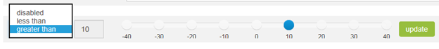
An example of the threshold selector.
For some engineering applications (and others), the use of percentile amounts is required. These values are available under the top menu variable drop-down selector. For example: ‘Percentile: maximum temperature’ is found under the main Temperature menu.
To obtain the actual percentile values, once the variable is selected the slider must be adjusted to the percentile desired (zero to 100) and UPDATE must be clicked. Percentiles are available at 0.5 unit intervals. The annual percentile amount is shown as is the historical trend for the selected period. Future percentiles are planned for the next CCHIP version.

An example of the percentile selector.
For temperature and precipitation variables, it is possible to display the historical distribution of daily values, allowing one to see the entire range and frequency of observations. Distributions such as these may be useful for users interested in further statistical analysis, for input into Monte-Carlo modelling or investigation of extreme value occurrence historically. Projected distributions are in development. Along with the histogram, a summary table is also provided.
Number of data points: 21972
min: -31.3
25th percentile: -3.4
mean: 5.87
stddev: 12.21
median: 7
75th percentile: 16.4
max: 30
[a, b) means an interval including a and up-to-but-not-including b.
An example of histogram summary table.
If a projection is available for a particular variable and data source, figures will be provided for the following baseline and future time horizons: 1981-2010 historical average figure, 2020s (2011-2040) ensemble average, 2050s (2041-2070) ensemble average, 2080s (2071-2100) ensemble average.
Typically, projection figures will only be available for stations with near-complete data for the baseline period of 1981-2010. Short station records do not provide projections since they have insufficient data for use in calculating the baseline climate.
The incident analysis tool is useful in exploring and determining factors that could have contributed to or caused identified impact events (incidents), at a specific location and on a specific date, using daily data. Short-term historical temperature and precipitation records (antecedent days prior to the incident), are readily provided for further analysis. The incident analysis feature also incorporates codes and standards values (design thresholds) stored or computed by CCHIP. Currently CCHIP provides these threshold values for all National Building Code of Canada 2015 variables, as well as for select variables from numerous other national codes and standards of Canada. Users may select from among the available climate thresholds and plot them together with the historical daily conditions, for user-specified time periods preceding the occurrence of the identified incident up to 30 days preceding.

An example of the incident analysis selector.
This feature will allow the system to provide news of and design-relevant information on extreme weather events. Currently there is an example of a Halifax roof collapse. On this page CCHIP also provides a link to a current Google News page with Canadian weather events.
Similar to the daily incident analysis view, this specific page is tailored to display hourly or custom datasets the system can ingest. Currently hourly data are available for select Canadian airport locations. Users may request further hourly data for their investigation by contacting us. Hourly data may only be displayed for the previous 10 days from the entered incident date.
The probability of frost profile is the daily probability of the occurrence of frost, i.e. when minimum temperature is less than 0°C, averaged over the 30-year period. It is expressed as the percentage of the number of days during the period when minimum temperature is less than 0°C and for plotting purposes, a five-day running mean has been applied to the data. An indication of the length of the freeze-free season is also given, i.e. the number of days during the year when the daily mean temperature is greater than 0°C.
Degree days are the accumulated departures of temperature above or below a particular threshold value, with these values selected to be of relevance to particular sectors, e.g. energy and agriculture. For example, a threshold temperature of 18°C is used as an indication of space heating or cooling requirements. For space heating, if the mean temperature is below 18°C then the departure from this threshold value is calculated and summed for all days on which the mean temperature is below the threshold value. For space cooling, the temperature departures are accumulated if the mean temperature on a particular day is above the 18°C threshold value. For growing seasons, threshold values commonly used here are 0°C, 5°C and 10°C.
Crop Heat Units (Brown, 1979; Bhartendu, 1984) were calculated between the start (mean daily temperature > 12.8°C for corn for 3 consecutive days during the period May 1st to July 31st) and end (first occurrence when minimum daily temperature is < -2°C during the period August 1st to October 15th) of the crop growing season.
For more information about crop heat unit, growing degree days and their calculations, please consults OMAFRA’s website here.
Freeze-thaw cycles represent the average number of days per period indicated when the daily maximum temperature equals or exceeds 0°C AND the daily minimum temperature is less than 0°C. The freeze-thaw cycle and its associated effects on water/ice formation can have significant effects on built environment deterioration.
The accumulated precipitation profile (in mm) indicates the progression of precipitation over a calendar year. Snow is converted to mm of water equivalent. The mean accumulation, maximum and minimum years for the period are shown as coloured lines. In addition, as an indication of extremes, diamonds indicate the progression of precipitation if either the maximum or minimum values of each month are summed for the period in question.
Monthly total precipitation, averaged over the 30-year period, is the rainfall amount plus the measured snowfall water equivalent. Actual and potential evapotranspiration values are also indicated. These have been derived from the Thornthwaite water balance calculations (Thornthwaite and Mather, 1955; Johnstone and Louie, 1983), an empirical method that computes changes in water storage as a function of monthly mean temperature, total precipitation, latitude (for day length) and soil texture (for water holding capacity). In the MacIver and Isaac (1989) study, all sites were assigned a soil water holding capacity of 100 mm, the value for sandy soils.
Water deficit and surplus are calculated from the potential and actual evapotranspiration values. Water deficit is the amount by which the available moisture fails to meet the demand for water and is computed by subtracting the potential evapotranspiration from the actual evapotranspiration for the period in question. Water surplus is the excess remaining after the evaporation needs of the soil have been met (i.e. when actual evapotranspiration equals potential evapotranspiration) and soil storage has been returned to the water holding capacity level.
This profile accumulates historical precipitation beginning on April 1 and ending October 31 of each year in the selected period to generate the average condition. Based upon standard deviation differences from this average condition colour bands indicate the departure from this normal condition. The standard deviation categories for the drought (drier than average) and flood (wetter than average) are 0.5, 1.0, 1.5 and 2.0. The average condition is shown by the thick dashed black line. The historical driest and wettest years in the period are also displayed, along with the user selected year which may be plotted to compare a particular year against normal conditions.
The use of the CCHIP tool is not to be considered free of error and caution is recommended in the interpretation of results. See the General Statement section below. RSI can provide expert advice and interpretation prior to any final implementation of results. Please contact us for assistance and guidance. The licenced CCHIP includes this assistance.
Every effort has been made to ensure the data used within CCHIP and the results it provides are as reliable as possible, however, data errors are possible. Neither RSI, nor CCHIP developers can guarantee the accuracy of the information presented. Please contact us with any questions arising from your analysis. Often spurious results can be attributed to missing data within the period being investigated. CCHIP allows the user to see how much data is missing in the information box beneath the charts.
This station has missing days for one or more years.
Click here to show/hide the full information.
Incomplete data warning.
RSI shall not be liable for any design, performance or other fault or defect in the use of this tool or for damages, costs, expenses or claims arising from or related to use of the CCHIP tool.
Clients will at all times indemnify RSI, and its staff from and against all claims, losses, damages, costs, expenses, actions and other proceedings made, sustained, brought, prosecuted or threatened in any manner based upon, caused by or in any way attributable to the use of the CCHIP tool.
Raw climatological data for Canada is provided by Environment and Climate Change Canada (ECCC) (www.ec.gc.ca), or gridded historical data (CANGRD) from Natural Resources Canada/ECCC.
National Building Code of Canada data is provided from the National Research Council (www.nrc-cnrc.gc.ca). Additional content is provided courtesy of the Standards Council of Canada (www.scc.ca).
Crop information is provided by various sources and is listed with the specific crop information page.
Projection data is provided from the IPCC (Intergovernmental Panel on Climate Change), the PCMDI (Program for Climate Model Diagnosis and Intercomparison), World Climate Research Program (WCRP), and CMIP (Coupled Model Intercomparison Project - phase 5 - (AR5)), has provided access to the international global climate model (GCM) data which is used in the production of ensemble projections within this tool. Use of the GCM data presented should acknowledge the provision of this raw data:
GCM data is provided by international modelling groups to the CMIP5 database (with support of the U.S. Department of Energy), with further analysis by Risk Sciences International (RSI) through the CCHIP.CA web tool.
Yes, after entering in a town near your station of interest, in the top right you can select a specific station from the dropdown or from the map of stations. The data will be updated with the new station you select
The data period shown next to each station shows the period of ‘any’ data. Not all variables. So it is possible to have, for example, temperature data for the period you want, but not precipitation which you may have selected at the moment. If you do need precipitation data, you should select another nearby station from the dropdown or map of stations.
The IDF station data shown is updated from Environment and Climate Change Canada at semi-regular intervals and represents the most recent available. Many stations over time have actually closed so it is quite possible to have IDF data which ended many years ago. There is no set date for the ECCC update of IDF station data.
Usually a very different year is the result of missing data during that year. For example, for an annual plot, if there was a significant period of missing summer data, that year would be ‘cold’. To assist in interpreting these issues, beneath the graph is a red box which provides a count of missing days in that year. Ideally the missing day counts per year should be minimal – but if not, this can influence the value plotted. Users are always advised to check for years with missing data (noted by ‘*’ next to the year on the plot), to see just how much data is missing.
Correct. CCHIP will plot a simple linear trend line fit through the data (it can be also toggled off if desired). At this time CCHIP does not have higher-order trend plotting. Also note that the tool does not provide a measure of significance of these linear trends – simply the equation and correlation coefficient (r2). For further detailed statistical analysis, the user is advised to download the data (from the ‘export’ link in the top right), and then import this CSV file into their preferred statistical or spreadsheet software.
No. At this time the user must select either one or the other with the radio button above the chart. This is easy however to toggle between and the actual values of the bars (historical and projected) can be exactly determined from either downloading the chart data (top right under ‘export’), or for a quick look, simply ‘mouse-over’ the bar and the value is displayed.
The short answer is you cannot at this time. CCHIP is developed to ensemble all available CMIP5 models to obtain the mean climate change signal from all. At this time there is no way to select a sub-set of these models for a different projection image. However, the individual model values can be seen on the boxplots and downloaded from the link beneath the boxplot.
This typically occurs if the baseline period (historical data record) is TOO short. For the best representation of historical climate, a record of 30 years is recommended. Shorter records may not reflect an accurate baseline which is required to produce a meaningful projection using the ‘delta approach’ we employ. In this case you should select another longer-record station nearby.
The variables list includes all variables on the system, but not necessarily those available at your selected station. For example, the IDF data is only available at stations noted with ‘+IDF’ in their names. Additionally, some variables like ‘visibility’ are only available for hourly data – which would be at airport locations. Hourly data can be accessed under the ‘hourly + incident analysis’ dashboard menu.
This is possible – but this is also calculable from the annual temperature plot if you download the annual data using the ‘export’ option in the top right. From there, you may sort the data and obtain the mean of the 3 coldest and mean of the 3 warmest years. As a test, we have added these 2 variables under the infrastructure option. Users can always contact us for variables which would be useful for their interests for consideration.
No. For efficiency, all of our chart generation uses the same template of colours/fonts and this is not modifiable. Do let us know if there is an issue you think we could improve. The only option at this time for truly customized charts for your use would be to use the ‘export’ function for the chart you have on the display and import that data into your favorite spreadsheet program for full customization of axes, colours, etc.
‘NaN’ is an acronym for ‘not a number’ and indicates an undefined value for that year (probably due to missing data). If not enough data is present for that year, then this is the result.
Not at this time. The 30 year periods shown on CCHIP are the ‘standard’ future 30-year periods used most often for climate change analysis. CCHIP continues to be developed however, and as part of this development we are investigating the use of different shorter projection periods. Any change will be noted in the ‘Updates’ section of the website (top menu item).
There is some text available about this on the rankings page itself, but basically you should be considering climate change no matter what your ranking score shows. The rankings are based upon percentile projected changes in the 2050s under RCP8.5 from across Canada. The greatest changes (rank 1) are found in Canadas Arctic with smaller changes in the south. The scores shown for temperature and precipitation are meant to show you where your location ranks in relation to the entire country. Those with higher scores will have the greatest impacts, but this does not imply that lower scoring locations will have NO impacts!
The year displayed for the winter value is the DECEMBER year. So the ‘Winter’ value for 1993 for example, would be December 1993 and January 1994 and February 1994.
If you have a question and could not find the information you needed after consulting the user manual, feel free to contact us via the Contact Us link at the top of the page, or email us at: cchip@risksciences.com.
Bhartendu, S. (1984): A Climatology of Corn Heat Units in Ontario. Ontario Region, Atmospheric Environment Service. Internal Report, SSD-84-1.
Brown, D.M. (1979): Heat Units for Corn in Southern Ontario. The Ontario Ministry of Agriculture and Food. Order No. 78-063.
Canadian Climate Impact Scenarios Project (2002): Bio-climate Profiles. http://www.cics.uvic.ca/scenarios/bcp/select.cgi.
IPCC-TGICA (2007). General Guidelines on the Use of Scenario Data for Climate Impact and Adaptation Assessment. Version 2. Prepared by T.R. Carter on behalf of the Intergovernmental Panel on Climate Change, Task Group on Data and Scenario Support for Impact and Climate Assessment, 66pp.
Johnstone, K. and P.Y.T. Louie (1983): Water Balance Tabulations for Canadian Climate Stations. Canadian Climate Centre, Environment Canada. 8-83. 14 pp.
Kharin, V. V., F. W. Zwiers, X. Zhang and M. Wehner (2013) Changes in temperature and precipitation extremes in the CMIP5 ensemble. Climatic Change. Vol. 119. No.2. pp 345-357.
MacIver, D.C. (1986): Climatograms by soil type for Ontario. In: Climate Applications in Forest Renewal and Forest Production, Proceedings of Forest Climate ’86, Canadian Forestry Service, Ottawa.
MacIver, D.C. and J.L. Isaac (1989): Bioclimate Profiles for Canada 1951-1980. Environment Canada, Atmospheric Environment Service.
MacIver, D.C. and B. Whitewood (1992): Forest Climates of Ontario: Part 1: Bioclimate Profiles 1968-88. Environment Canada, Atmospheric Environment Service.
McKenney, D. W. et al. 2011. Customized Spatial Climate Models for North America. Bull. American Meteorological Soc. V 92 (12). Pp 1611-1622.
Tebaldi, C. and R. Knutti (2007). The use of the multimodel ensemble in probabilistic climate projections. Philosophical Transactions of the Royal Society (special issue on Probabilistic Climate Change Projections), Vol. 365, pp. 2053-2075.
Thornthwaite, C.W. and J.R. Mather (1955). The Water Balance. Drexel Institute of Technology. Publications in Climatology 8(1).